Principal Component Analysis Solved Example
Principal component analysis (PCA) is a statistical procedure that uses an orthogonal transformation to convert a set of observations of possibly correlated variables into a set of values of linearly uncorrelated variables called principal components.
In this article, I will discuss how to find the principal components with a simple solved numerical example.
Video Tutorial Principle Component Analysis – Dimensionality Reduction in Machine Learning
PCA Video Tutorial
Problem definition
Given the data in Table, reduce the dimension from 2 to 1 using the Principal Component Analysis (PCA) algorithm.
| Feature | Example 1 | Example 2 | Example 3 | Example 4 |
| X1 | 4 | 8 | 13 | 7 |
| X2 | 11 | 4 | 5 | 14 |
Step 1: Calculate Mean
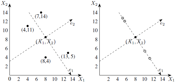
The figure shows the scatter plot of the given data points.

Calculate the mean of X1 and X2 as shown below.

Step 2: Calculation of the covariance matrix.
The covariances are calculated as follows:

The covariance matrix is,

Step 3: Eigenvalues of the covariance matrix
The characteristic equation of the covariance matrix is,

Solving the characteristic equation we get,

Step 4: Computation of the eigenvectors
To find the first principal components, we need only compute the eigenvector corresponding to the largest eigenvalue. In the present example, the largest eigenvalue is λ1 and so we compute the eigenvector corresponding to λ1.
The eigenvector corresponding to λ = λ1 is a vector

satisfying the following equation:

This is equivalent to the following two equations:

Using the theory of systems of linear equations, we note that these equations are not independent and solutions are given by,

that is,

where t is any real number.
Taking t = 1, we get an eigenvector corresponding to λ1 as

To find a unit eigenvector, we compute the length of X1 which is given by,

Therefore, a unit eigenvector corresponding to λ1 is

By carrying out similar computations, the unit eigenvector e2 corresponding to the eigenvalue λ= λ2 can be shown to be,

Step 5: Computation of first principal components
let,

be the kth sample in the above Table (dataset). The first principal component of this example is given by (here “T” denotes the transpose of the matrix)

For example, the first principal component corresponding to the first example

is calculated as follows:

The results of the calculations are summarised in the below Table.
| X1 | 4 | 8 | 13 | 7 |
| X2 | 11 | 4 | 5 | 14 |
| First Principle Components | -4.3052 | 3.7361 | 5.6928 | -5.1238 |
Step 6: Geometrical meaning of first principal components
First, we shift the origin to the “center”

and then change the directions of coordinate axes to the directions of the eigenvectors e1 and e2.

Next, we drop perpendiculars from the given data points to the e1-axis (see below Figure).

The first principal components are the e1-coordinates of the feet of perpendiculars, that is, the projections on the e1-axis. The projections of the data points on the e1-axis may be taken as approximations of the given data points hence we may replace the given data set with these points.
Now, each of these approximations can be unambiguously specified by a single number, namely, the e1-coordinate of
approximation. Thus the two-dimensional data set can be represented approximately by the following one-dimensional data set.

Summary: Principal Component Analysis Solved Example
This article discusses what is Principal component analysis in Machine Learning and how to find the Principal Components using the PCA algorithm – Solved Example. If you like the material share it with your friends. Like the Facebook page for regular updates and the YouTube channel for video tutorials.
